model-compression-and-acceleration.md

An Overview of Model Compression and Acceleration
Author:Jet Date:2023/07

Background

1. 减少模型存储和计算成本

2. 期望模型不仅能部署在服务端GPU，也能部署在移动端

3. 神经网络中卷积层、全连接层权重参数具有冗余的特点

   卷积层占据了大约 90-95% 的计算时间和参数规模，有较大的值；全连接层占据了大约 5-10% 的计算时间，95% 的参数规模，并且值较小

Related work

​ 综合现有的深度模型压缩方法，它们主要分为四类:

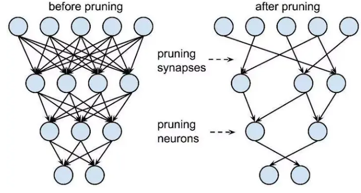
• 参数剪枝和共享（parameter pruning and sharing）
  • 针对模型参数的冗余性，试图去除冗余和不重要的项
• 低秩因子分解（low-rank factorization）
  • 使用矩阵/张量分解来估计深度学习模型的信息参数
• 转移/紧凑卷积滤波器（transferred/compact convolutional filters）
  • 特殊的结构卷积滤波器来降低存储和计算复杂度
• 知识蒸馏（knowledge distillation）
  • 训练一个更紧凑的神经网络来重现一个更大的网络的输出

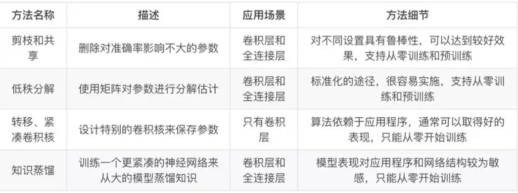
​ 一般来说，参数修剪和共享，低秩分解和知识蒸馏方法可以用于全连接层和卷积层的 CNN，但另一方面，使用转移/紧凑型卷积核的方法仅支持卷积层。低秩因子分解和基于转换/紧凑型卷积核的方法提供了一个端到端的流水线，可以很容易地在 CPU/GPU 环境中实现。相反参数修剪和共享使用不同的方法，如矢量量化，二进制编码和稀疏约束来执行任务，这导致常需要几个步骤才能达到目标。

​ 基于参数修剪/共享、低秩分解的模型可以从预训练模型或者从头开始训练，因此灵活而有效。然而转移/紧凑的卷积核和知识蒸馏模型只能支持从零开始训练。

参数修剪和共享

​ 三类：模型量化和二进制化、参数共享和结构化矩阵（structural matrix）

• 网络量化(quantization)通过减少表示每个权重所需的比特数来压缩原始网络：fp32 fp16 int8 int4
• 修剪减少了需要编码的权重数量，量化和霍夫曼编码减少了用于对每个权重编码的比特数。对于大部分元素为 0 的矩阵可以使用稀疏表示，进一步降低空间冗余，且这种压缩机制不会带来任何准确率损失。
• 剪枝:

低秩分解和稀疏性

​ 典型的 CNN 卷积核是一个 4D 张量，而全连接层也可以当成一个 2D 矩阵，低秩分解同样可行。这些张量中可能存在大量的冗余。所有近似过程都是逐层进行的，在一个层经过低秩滤波器近似之后，该层的参数就被固定了，而之前的层已经用一种重构误差标准（reconstruction error criterion）微调过。

迁移/压缩卷积滤波器

​ 在 Inception 结构中使用了将 3×3 卷积分解成两个 1×1 的卷积；SqueezeNet 提出用 1×1 卷积来代替 3×3 卷积，与 AlexNet 相比，SqueezeNet 创建了一个紧凑的神经网络，参数少了 50 倍，准确度相当。

知识蒸馏

​ “学生-教师”的范式，即通过软化“教师”的输出而惩罚“学生”

​ 只能用于具有 Softmax 损失函数分类任务

TensorFlow 支持的是一种静态图，当模型的参数确定之后，便无法继续修改。这对于逐阶段、分层的训练带来了一定的困难。相比之下，Pytorch 使用了动态图，在定义完模型之后还可以边训练边修改其参数，具有很高的灵活性。这也是深度学习未来的发展方向

YOLOv6

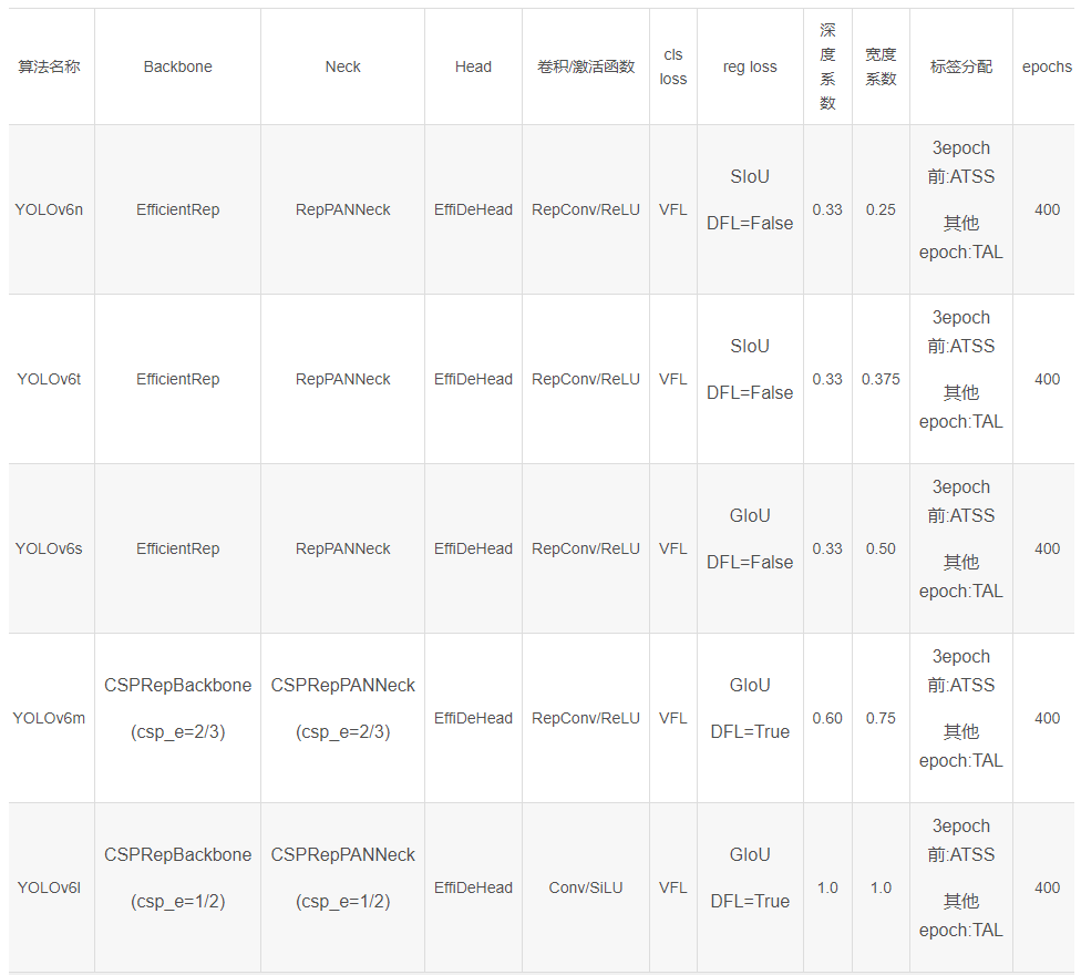
EfficientRep Backbone

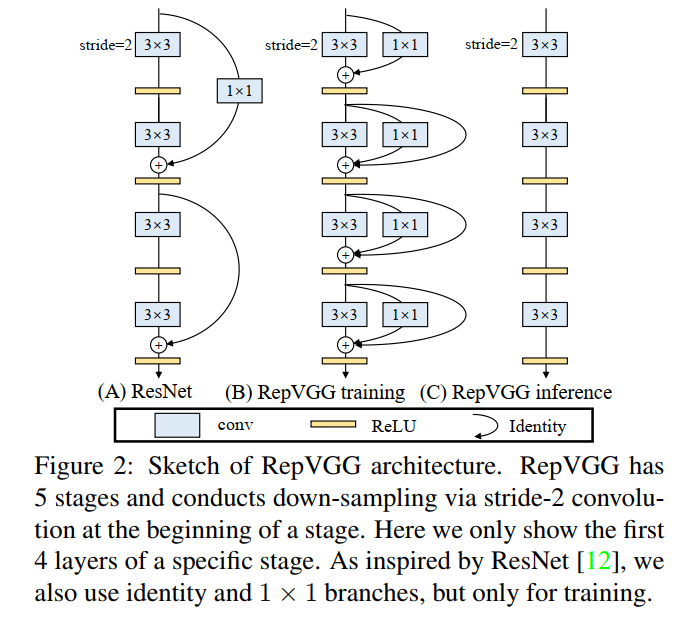
• 多分支的网络(ResNet,DenseNet,GoogLeNet)相比单分支(ImageNet,VGG)的通常能够有更好的分类性能。但是，它通常伴随着并行性的降低，并导致推理延迟的增加。相反，像VGG这样的普通单路径网络具有高并行性和较少内存占用的优点，从而导致更高的推理效率。
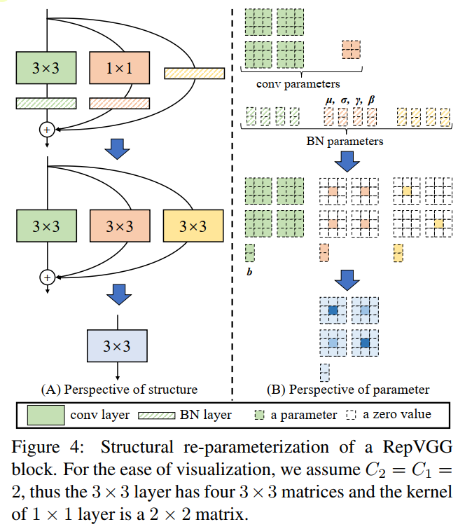
• RepVGG Style 结构是一种在训练时具有多分支拓扑，而在实际部署时可以等效融合为单个 3x3 卷积的一种可重参数化的结构。通过融合成的 3x3 卷积结构，可以有效利用计算密集型硬件计算能力（比如 GPU），同时也可获得 GPU/CPU 上已经高度优化的 NVIDIA cuDNN 和 Intel MKL 编译框架的帮助。

Rep-PAN neck

• 将YOLOv5中使用的 CSPBlock替换为RepBlock（适用于小型模型）或CSPStackRep Block（用于大型模型），并相应调整宽度和深度。

Decoupled Head

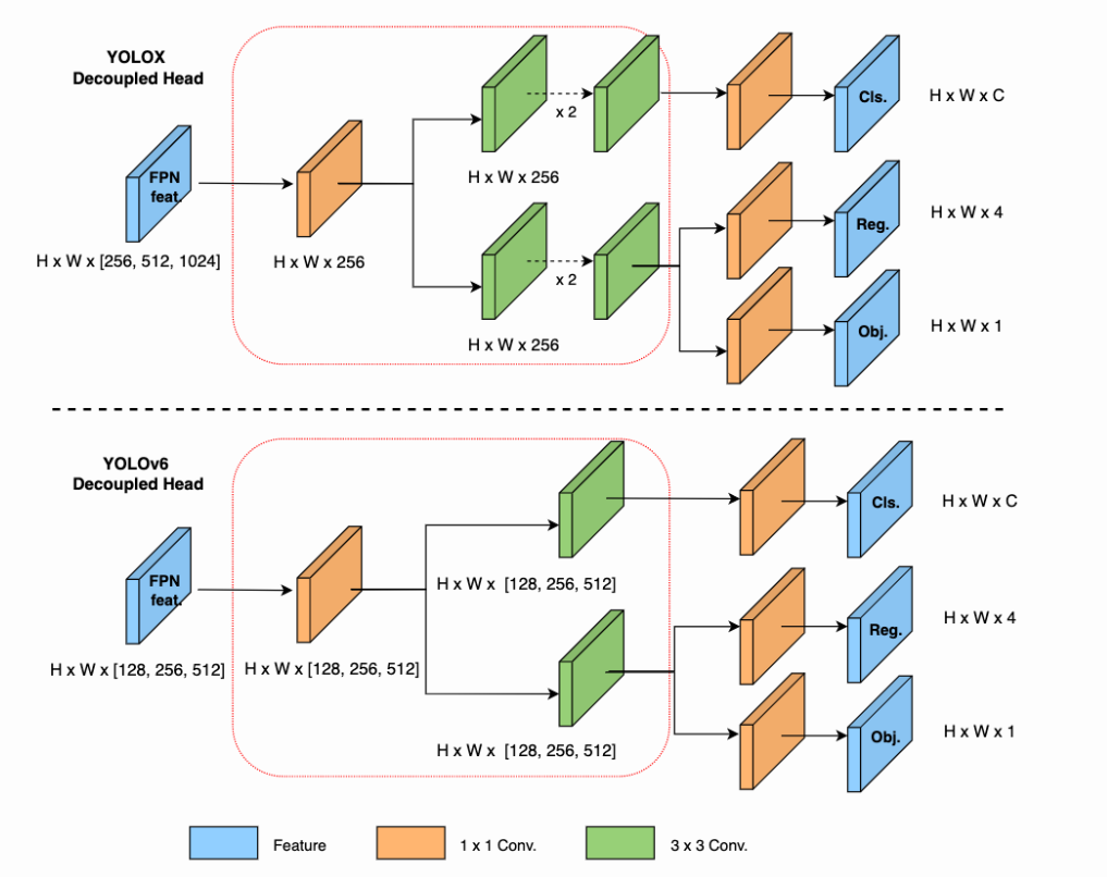
• 原始 YOLOv5 的检测头是通过分类和回归分支融合共享的方式来实现的，而 YOLOX 的检测头则是将分类和回归分支进行解耦，同时新增了两个额外的 3x3 的卷积层，虽然提升了检测精度，但一定程度上增加了网络延时。

• 因此，我们对解耦头进行了精简设计，同时综合考虑到相关算子表征能力和硬件上计算开销这两者的平衡，采用 Hybrid Channels 策略重新设计了一个更高效的解耦头结构，在维持精度的同时降低了延时，缓解了解耦头中 3x3 卷积带来的额外延时开销。通过在 nano 尺寸模型上进行消融实验，对比相同通道数的解耦头结构，精度提升 0.2% AP 的同时，速度提升6.8%。

Training strategies

Anchor-free

• 由于 Anchor-based检测器需要在训练之前进行聚类分析以确定最佳 Anchor 集合，这会一定程度提高检测器的复杂度；同时，在一些边缘端的应用中，需要在硬件之间搬运大量检测结果的步骤，也会带来额外的延时。而 Anchor-free 无锚范式因其泛化能力强，解码逻辑更简单，在近几年中应用比较广泛。经过对 Anchor-free 的实验调研，我们发现，相较于Anchor-based 检测器的复杂度而带来的额外延时，Anchor-free 检测器在速度上有51%的提升。有两种类型的anchor-free检测器：point-based(YOLOX,FCOS)和keypoing-based(CenterNet)。在YOLOv6中，采用了 anchor-free point-based范式。

TAL

• OTA将目标检测中的标签分配视为最佳传输的问题。它从全局角度定义了每个GT目标的正/负训练样本。SimOTA是OTA的简化版本，它减少了额外的超参数并保持了性能。在YOLOv6的早期版本中，SimOTA被用作标签分配方法。然而，在实践中，发现引入SimOTA会减缓训练过程。而且，陷入不稳定训练的情况经常出现。因此，设计了一个 SimOTA的替代品TAL。

• Task alignment learning：任务对齐学习（TAL），TOOD: Task-aligned One-stage Object Detection任务对齐的单阶段目标检测。由于分类和定位的学习机制不同，两个任务学习到的特征的空间分布可能不同，当使用两个单独的分支进行预测时，会导致一定程度的错位。增加两个任务之间的交互，(2)增强检测器学习比对的能力

Activation

• YOLO系列激活函数各不相同，如ReLU、LReLU、Swish、SiLU、Mish等。在这些激活函数中，SiLU是使用最多的。一般来说，SiLU的精度更高，不会造成太多额外的计算成本。然而，在工业应用中，特别是在部署具有TensorRT加速的模型时，ReLU具有更大的速度优势，因为它融合到了卷积中。

• 此外，进一步验证了RepConv/普通卷积（表示为Conv）和ReLU/SiLU/LReLU组合在不同大小网络中的有效性，以实现更好的折衷。带有SiLU的Conv在精度上表现最佳， 而RepConv和ReLU的组合实现了更好的权衡。所以建议用户在对延迟敏感的应用程序中使用RepConv和ReLU。

• 使用RepConv/ReLU在YOLOv6-N/T/S/M中，用于更高的推理速度；在大型型号 YOLOv6-L中使用Conv/SiLU组合加速训练并提高性能

Loss

• Classification Loss

  • Focal Loss修改了传统的交叉熵损失，以解决正负样本或难易样本之间的类不平衡问题。为了解决训练和推理之间质量估计和分类的不一致使用，Quality Focal Loss（QFL）进一步扩展了Focal Loss，将分类分数和本地化质量联合表示用于分类监督。而VariFocal Loss（VFL）源于Focal Loss，但它不对称地处理正样本和负样本。通过考虑不同重要程度的正样本和负样本，它平衡了来自两个样本的学习信号。Poly Loss将常用的分类损失分解为一系列加权多项式基。它在不同的任务和数据集上调整多项式系数，通过实验证明其优于交叉熵损失和Focal Loss
    • 在YOLOv6-N/S/M上实验了Focal Los、Polyloss、QFL和VFL。如表8所示，与Focal Loss相比，VFL对YOLOv6-N/S/M分别带来0.2%/0.3%/0.1%的AP改善。所以，选择 VFL作为分类损失函数

• Box Regression Loss

  ​ 框回归损失为精确定位边界盒提供了重要的学习信号。L1 Loss是早期工作中的原始框回归损失。逐渐地，各种精心设计的框回归损失如IoU系列Loss和Probability Loss如雨后春笋般涌现。

  • IoU-series Loss： IoU Loss将预测框的四个边界作为一个整体单位进行回归。由于其与评价指标的一致性，已被证明是有效的。IoU有许多变体，如GIoU、DIoU、CIoU、α-IoU和SIoU等，形成相关损失函数。对GIoU、CIoU和SIoU进行了实验。 SIoU应用于YOLOv6-N和YOLOV 6-T，而其他的使用GIoU

    • 对于 YOLOv6-N和YOLOv 6-T，SIoU Loss优于其他Loss，而对于 YOLOv6-M，CIoU Loss表现更好

  • Probability Loss

    • Dostronition Focal Loss（DFL）将框位置的基本连续分布简化为离散化概率分布。**它考虑了数据中的模糊性和不确定性，而不引入任何其他先验，这有助于提高框定位精度，特别是当GT框的边界模糊时。基于DFL，DFLv2开发了一个轻量级子网络，以利用分布统计和实际定位质量之间的密切相关性，进一步提高检测性能。然而，DFL通常输出比一般盒回归多17倍的回归值，导致大量开销。额外的计算成本显著阻碍了小模型的训练。
    • 仅在YOLOv6-M/L中采用DFL

  • Object Loss

    • FCOS中首次提出了Object Loss，以降低低质量边界框的分数，以便在后处理中过滤掉它们。在YOLOX中也使用了它来加速收敛并提高网络精度。作为一个像FCOS和YOLOX这样的anchor-free框架，本文尝试将Object Loss引入YOLOv6。不幸的是，它没有带来很多积极的效果。
    • 在 YOLOv6中去除Object Loss

Epochs

• 随着训练时间的增加，检测器的性能不断提高。我们将训练时间从300个周期延长到400个周期，以达到更好的收敛。

Self-distillation

• 在评估YOLOv5和YOLOv7中的模型性能时，在每个图像周围放置了half-stride灰色边界（就是resize图片时四周填充了灰度的padding）。虽然没有添加有用的信息，但它有助于检测图像边缘附近的对象。这个技巧也适用于YOLOv6
• 然而，额外的灰度像素明显降低了推理速度。如果没有灰色边界，YOLOv6的性能会恶化，这也是YOLOv5和YOLOv7中遇到的情况。我们假设该问题与Mosaic增强中的灰色边界填充有关。为了验证，进行了在最后一个epoch时关闭Mosaic增强的实验（又名衰退策略,fade strategy）。在这方面，我们改变了灰度边界的面积，并将具有灰度边界的图像直接调整为目标图像大小。结合这两种策略，我们的模型可以在不降低推理速度的情况下保持甚至提高性能
• 一方面，性能下降的问题得到了缓解。另一方面，无论是否填充灰色边界，小模型（YOLOv6-N/S）的精度都会提高
• 将输入图像限制为634×634，并在边缘周围添加3像素宽的灰色边界。使用该策略，最终图像的大小为预期的640×640。当最终图像尺寸从672减小到640时，YOLOv6-N/S/M的最终性能甚至更精确0.2%/0.3%/0.1%

Methodology

• https://github.com/meituan/YOLOv6/blob/main/docs/tutorial_repopt.md
  • step 1 Training with RepOptimizer
  • step 2 PTQ + sensitivity analyze
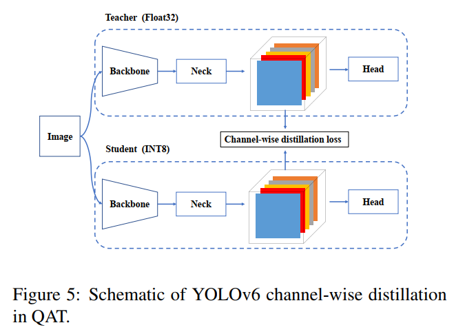
  • step 3 QAT: channel-wise distillation

RepOptimizers

​ 重参数化优化器, 针对VGG这种结构进行优化

​ 将先验信息用于修改梯度数值，称为梯度重参数化，对应的优化器称为RepOptimizer。我们着重关注VGG式的直筒模型，训练得到RepOptVGG模型，他有着高训练效率，简单直接的结构和极快的推理速度。

• paper https://arxiv.org/pdf/2205.15242.pdf

• code https://github.com/DingXiaoH/RepOptimizers

  • https://zhuanlan.zhihu.com/p/531477704

• 与RepVGG的区别

1. RepVGG加入了结构先验（如1x1，identity分支），并使用常规优化器训练。而RepOptVGG则是将这种先验知识加入到优化器实现中
2. 尽管RepVGG在推理阶段可以把各分支融合，成为一个直筒模型。但是其训练过程中有着多条分支，需要更多显存和训练时间。而RepOptVGG可是 真-直筒模型，从训练过程中就是一个VGG结构
3. 我们通过定制优化器，实现了结构重参数化和梯度重参数化的等价变换，这种变换是通用的，可以拓展到更多模型

• https://github.com/meituan/YOLOv6/blob/main/docs/tutorial_repopt.md

  def quant_sensitivity_analyse(model_ptq, evaler):
      # disable all quantable layer
      model_quant_disable(model_ptq)
      
      # analyse each quantable layer
      quant_sensitivity = list()
      for k, m in model_ptq.named_modules():
          if isinstance(m, quant_nn.QuantConv2d) or \
             isinstance(m, quant_nn.QuantConvTranspose2d) or \
             isinstance(m, quant_nn.MaxPool2d):
              module_quant_enable(model_ptq, k)
          else:
              # module can not be quantized, continue
              continue
  
          eval_result = evaler.eval(model_ptq)
          print(eval_result)
          print("Quantize Layer {}, result mAP0.5 = {:0.4f}, mAP0.5:0.95 = {:0.4f}".format(k,
                                                                                            eval_result[0],
                                                                                            eval_result[1]))
          quant_sensitivity.append((k, eval_result[0], eval_result[1]))
          # disable this module sensitivity, anlayse next module
          module_quant_disable(model_ptq, k)
  
      return quant_sensitivity

• EfficientRep：An Efficient Repvgg-style ConvNets with Hardware-aware Neural Network Design

  • https://arxiv.org/abs/2302.00386

  backbone=dict(
      type='EfficientRep',
      num_repeats=[1, 6, 12, 18, 6],
      out_channels=[64, 128, 256, 512, 1024],
      ),
  neck=dict(
      type='RepPANNeck',
      num_repeats=[12, 12, 12, 12],
      out_channels=[256, 128, 128, 256, 256, 512],
      ),
  head=dict(
      type='EffiDeHead',
      in_channels=[128, 256, 512],
      num_layers=3,
      begin_indices=24,
      anchors=1,
      out_indices=[17, 20, 23],
      strides=[8, 16, 32],
      atss_warmup_epoch=0,
      iou_type='giou',
      use_dfl=False,
      reg_max=0
  )

• 用了RepVGGOptimizer SGD针对VGGBlock进行优化

  • https://github.com/meituan/YOLOv6/blob/main/yolov6/utils/RepOptimizer.py
  • https://github.com/DingXiaoH/RepOptimizers/blob/main/repoptimizer/repoptvgg_impl.py
  • 不同的优化器SGD AdamW配置不同
    • In the step function, RepOptimizers will use the Grad Mults properly. For SGD, please see here. For AdamW, please see here and here.

  from ..layers.common import RealVGGBlock, LinearAddBlock
  def extract_blocks_into_list(model, blocks):
     for module in model.children():
          if isinstance(module, LinearAddBlock) or isinstance(module, RealVGGBlock):
              blocks.append(module)
          else:
              extract_blocks_into_list(module, blocks)

  class RepVGGOptimizer(SGD):
      '''scales is a list, scales[i] is a triple (scale_identity.weight, scale_1x1.weight, scale_conv.weight) or a two-tuple (scale_1x1.weight, scale_conv.weight) (if the block has no scale_identity)'''
      def __init__(self, model, scales,
                   args, cfg, momentum=0, dampening=0,
                   weight_decay=0, nesterov=True,
                   reinit=True, use_identity_scales_for_reinit=True,
                   cpu_mode=False):
  
          defaults = dict(lr=cfg.solver.lr0, momentum=cfg.solver.momentum, dampening=dampening, weight_decay=weight_decay, nesterov=nesterov)
          if nesterov and (cfg.solver.momentum <= 0 or dampening != 0):
              raise ValueError("Nesterov momentum requires a momentum and zero dampening")
          # parameters = set_weight_decay(model)
          parameters = get_optimizer_param(args, cfg, model)
          super(SGD, self).__init__(parameters, defaults)
          self.num_layers = len(scales)
  
          blocks = []
          extract_blocks_into_list(model, blocks)
          convs = [b.conv for b in blocks]
          assert len(scales) == len(convs)
  
          if reinit:
              for m in model.modules():
                  if isinstance(m, nn.BatchNorm2d):
                      gamma_init = m.weight.mean()
                      if gamma_init == 1.0:
                          LOGGER.info('Checked. This is training from scratch.')
                      else:
                          LOGGER.warning('========================== Warning! Is this really training from scratch ? =================')
              LOGGER.info('##################### Re-initialize #############')
              self.reinitialize(scales, convs, use_identity_scales_for_reinit)
  
          self.generate_gradient_masks(scales, convs, cpu_mode)
  
      def reinitialize(self, scales_by_idx, conv3x3_by_idx, use_identity_scales):
          for scales, conv3x3 in zip(scales_by_idx, conv3x3_by_idx):
              in_channels = conv3x3.in_channels
              out_channels = conv3x3.out_channels
              kernel_1x1 = nn.Conv2d(in_channels, out_channels, 1, device=conv3x3.weight.device)
              if len(scales) == 2:
                  conv3x3.weight.data = conv3x3.weight * scales[1].view(-1, 1, 1, 1) \
                                        + F.pad(kernel_1x1.weight, [1, 1, 1, 1]) * scales[0].view(-1, 1, 1, 1)
              else:
                  assert len(scales) == 3
                  assert in_channels == out_channels
                  identity = torch.from_numpy(np.eye(out_channels, dtype=np.float32).reshape(out_channels, out_channels, 1, 1)).to(conv3x3.weight.device)
                  conv3x3.weight.data = conv3x3.weight * scales[2].view(-1, 1, 1, 1) + F.pad(kernel_1x1.weight, [1, 1, 1, 1]) * scales[1].view(-1, 1, 1, 1)
                  if use_identity_scales:     # You may initialize the imaginary CSLA block with the trained identity_scale values. Makes almost no difference.
                      identity_scale_weight = scales[0]
                      conv3x3.weight.data += F.pad(identity * identity_scale_weight.view(-1, 1, 1, 1), [1, 1, 1, 1])
                  else:
                      conv3x3.weight.data += F.pad(identity, [1, 1, 1, 1])
  
      def generate_gradient_masks(self, scales_by_idx, conv3x3_by_idx, cpu_mode=False):
          self.grad_mask_map = {}
          for scales, conv3x3 in zip(scales_by_idx, conv3x3_by_idx):
              para = conv3x3.weight
              if len(scales) == 2:
                  mask = torch.ones_like(para, device=scales[0].device) * (scales[1] ** 2).view(-1, 1, 1, 1)
                  mask[:, :, 1:2, 1:2] += torch.ones(para.shape[0], para.shape[1], 1, 1, device=scales[0].device) * (scales[0] ** 2).view(-1, 1, 1, 1)
              else:
                  mask = torch.ones_like(para, device=scales[0].device) * (scales[2] ** 2).view(-1, 1, 1, 1)
                  mask[:, :, 1:2, 1:2] += torch.ones(para.shape[0], para.shape[1], 1, 1, device=scales[0].device) * (scales[1] ** 2).view(-1, 1, 1, 1)
                  ids = np.arange(para.shape[1])
                  assert para.shape[1] == para.shape[0]
                  mask[ids, ids, 1:2, 1:2] += 1.0
              if cpu_mode:
                  self.grad_mask_map[para] = mask
              else:
                  self.grad_mask_map[para] = mask.cuda()
  
      def __setstate__(self, state):
          super(SGD, self).__setstate__(state)
          for group in self.param_groups:
              group.setdefault('nesterov', False)
  
      def step(self, closure=None):
          loss = None
          if closure is not None:
              loss = closure()
  
          for group in self.param_groups:
              weight_decay = group['weight_decay']
              momentum = group['momentum']
              dampening = group['dampening']
              nesterov = group['nesterov']
  
              for p in group['params']:
                  if p.grad is None:
                      continue
  
                  if p in self.grad_mask_map:
                      d_p = p.grad.data * self.grad_mask_map[p]  # Note: multiply the mask here
                  else:
                      d_p = p.grad.data
  
                  if weight_decay != 0:
                      d_p.add_(weight_decay, p.data)
                  if momentum != 0:
                      param_state = self.state[p]
                      if 'momentum_buffer' not in param_state:
                          buf = param_state['momentum_buffer'] = torch.clone(d_p).detach()
                      else:
                          buf = param_state['momentum_buffer']
                          buf.mul_(momentum).add_(1 - dampening, d_p)
                      if nesterov:
                          d_p = d_p.add(momentum, buf)
                      else:
                          d_p = buf
  
                  p.data.add_(-group['lr'], d_p)
  
          return loss
  

Partial quantization

• https://github.com/meituan/YOLOv6/blob/main/tools/partial_quantization/sensitivity_analyse.py

先做参数敏感性分析，再对不敏感的参数进行量化

所谓参数敏感性，就是判断参数变化对性能是否影响，如果影响很大，则敏感，否则不敏感, 采用控制变量法进行逐层分析

评价指标是在数据集上测试mAP，mAP相对全精度变化大则认为敏感

最后做敏感度排序

def quant_sensitivity_analyse(model_ptq, evaler):
    # disable all quantable layer
    model_quant_disable(model_ptq)

    # analyse each quantable layer
    quant_sensitivity = list()
    for k, m in model_ptq.named_modules():
        if isinstance(m, quant_nn.QuantConv2d) or \
           isinstance(m, quant_nn.QuantConvTranspose2d) or \
           isinstance(m, quant_nn.MaxPool2d):
            module_quant_enable(model_ptq, k)
        else:
            # module can not be quantized, continue
            continue

        eval_result = evaler.eval(model_ptq)
        print(eval_result)
        print("Quantize Layer {}, result mAP0.5 = {:0.4f}, mAP0.5:0.95 = {:0.4f}".format(k,
                                                                                          eval_result[0],
                                                                                          eval_result[1]))
        quant_sensitivity.append((k, eval_result[0], eval_result[1]))
        # disable this module sensitivity, anlayse next module
        module_quant_disable(model_ptq, k)

    return quant_sensitivity

def module_quant_disable(model, k):
    cur_module = get_module(model, k)
    if hasattr(cur_module, '_input_quantizer'):
        cur_module._input_quantizer.disable()
    if hasattr(cur_module, '_weight_quantizer'):
        cur_module._weight_quantizer.disable()


def module_quant_enable(model, k):
    cur_module = get_module(model, k)
    if hasattr(cur_module, '_input_quantizer'):
        cur_module._input_quantizer.enable()
    if hasattr(cur_module, '_weight_quantizer'):
        cur_module._weight_quantizer.enable()

With partial quantization, we finally reach 42.1%, only 0.3% loss in accuracy, while the throughput of the partially quantized model is about 1.56 times that of the FP16 model at a batch size of 32. This method achieves a nice tradeoff between accuracy and throughput.

Pytorch quantization

• https://docs.nvidia.com/deeplearning/tensorrt/pytorch-quantization-toolkit/docs/index.html

  • https://github.com/Jermmy/pytorch-quantization-demo

• 自定义量化模块 https://docs.nvidia.com/deeplearning/tensorrt/pytorch-quantization-toolkit/docs/tutorials/creating_custom_quantized_modules.html

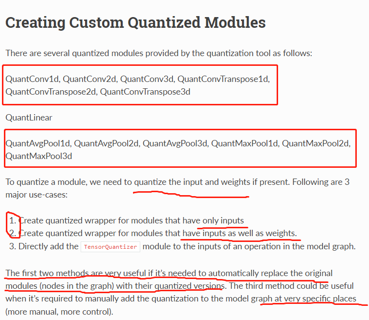
  • 主要是卷积层、反卷积层、池化层
  • 注意输入或者权重的量化封装情况，有的只量化输入，有的要量化输入和权重
  • 也可以自定义TensorQuantizer进行控制

• https://github.com/NVIDIA/TensorRT/blob/master/tools/pytorch-quantization/examples/torchvision/models/classification/resnet.py

if quantize:
    self.conv1 = quant_nn.QuantConv2d(3,
                                self.inplanes,
                                kernel_size=7,
                                stride=2,
                                padding=3,
                                bias=False)
else:
    self.conv1 = nn.Conv2d(3, self.inplanes, kernel_size=7, stride=2, padding=3, bias=False)

• https://github.com/Jermmy/pytorch-quantization-demo/blob/master/model.py#L34

  QAT需要对需要量化的层进行替换，比如QConv2d QReLU QMaxPooling2d QLinear，相当于用Q重构模型进行训练和推理，其中Qxx参考 https://github.com/Jermmy/pytorch-quantization-demo/blob/master/module.py （最好用官方的进行替换QuantConv2d，或者源码替换QConv2d）

  class Net(nn.Module):
  
      def __init__(self, num_channels=1):
          super(Net, self).__init__()
          self.conv1 = nn.Conv2d(num_channels, 40, 3, 1)
          self.conv2 = nn.Conv2d(40, 40, 3, 1, groups=20)
          self.fc = nn.Linear(5*5*40, 10)
  
      def forward(self, x):
          x = F.relu(self.conv1(x))
          x = F.max_pool2d(x, 2, 2)
          x = F.relu(self.conv2(x))
          x = F.max_pool2d(x, 2, 2)
          x = x.view(-1, 5*5*40)
          x = self.fc(x)
          return x
  
      def quantize(self, num_bits=8):
          self.qconv1 = QConv2d(self.conv1, qi=True, qo=True, num_bits=num_bits)
          self.qrelu1 = QReLU()
          self.qmaxpool2d_1 = QMaxPooling2d(kernel_size=2, stride=2, padding=0)
          self.qconv2 = QConv2d(self.conv2, qi=False, qo=True, num_bits=num_bits)
          self.qrelu2 = QReLU()
          self.qmaxpool2d_2 = QMaxPooling2d(kernel_size=2, stride=2, padding=0)
          self.qfc = QLinear(self.fc, qi=False, qo=True, num_bits=num_bits)
  
      def quantize_forward(self, x):
          x = self.qconv1(x)
          x = self.qrelu1(x)
          x = self.qmaxpool2d_1(x)
          x = self.qconv2(x)
          x = self.qrelu2(x)
          x = self.qmaxpool2d_2(x)
          x = x.view(-1, 5*5*40)
          x = self.qfc(x)
          return x
  
      def freeze(self):
          self.qconv1.freeze()
          self.qrelu1.freeze(self.qconv1.qo)
          self.qmaxpool2d_1.freeze(self.qconv1.qo)
          self.qconv2.freeze(qi=self.qconv1.qo)
          self.qrelu2.freeze(self.qconv2.qo)
          self.qmaxpool2d_2.freeze(self.qconv2.qo)
          self.qfc.freeze(qi=self.qconv2.qo)
  
      def quantize_inference(self, x):
          qx = self.qconv1.qi.quantize_tensor(x)
          qx = self.qconv1.quantize_inference(qx)
          qx = self.qrelu1.quantize_inference(qx)
          qx = self.qmaxpool2d_1.quantize_inference(qx)
          qx = self.qconv2.quantize_inference(qx)
          qx = self.qrelu2.quantize_inference(qx)
          qx = self.qmaxpool2d_2.quantize_inference(qx)
          qx = qx.view(-1, 5*5*40)
          qx = self.qfc.quantize_inference(qx)
          out = self.qfc.qo.dequantize_tensor(qx)
          return out

Post-training quantization (PTQ)

• https://github.com/meituan/YOLOv6/blob/main/tools/partial_quantization/ptq.py
• https://docs.nvidia.com/deeplearning/tensorrt/pytorch-quantization-toolkit/docs/userguide.html#post-training-quantization

QuantDescriptor 定义量化方法直方图，量化位数8bit，作为量化输入描述子

conv2d_weight_default_desc 作为权重量化描述子

针对Conv2d ConvTranspose2d MaxPool2d分别用相应的量化算子替代即可

PTQ只需迭代1-2epoch即可，而且是推理阶段（前向传播 with torch.no_grad()）

考虑敏感性分析，非敏感层可以用PTQ，敏感层不变，可以减少精度损失

def quant_model_init(model, device):
    model_ptq = copy.deepcopy(model)
    model_ptq.eval()
    model_ptq.to(device)
    conv2d_weight_default_desc = tensor_quant.QUANT_DESC_8BIT_CONV2D_WEIGHT_PER_CHANNEL
    conv2d_input_default_desc = QuantDescriptor(num_bits=8, calib_method='histogram')

    convtrans2d_weight_default_desc = tensor_quant.QUANT_DESC_8BIT_CONVTRANSPOSE2D_WEIGHT_PER_CHANNEL
    convtrans2d_input_default_desc = QuantDescriptor(num_bits=8, calib_method='histogram')

    for k, m in model_ptq.named_modules():
        if 'proj_conv' in k:
            print("Skip Layer {}".format(k))
            continue

        if isinstance(m, nn.Conv2d):
            in_channels = m.in_channels
            out_channels = m.out_channels
            kernel_size = 
            m.kernel_size
            stride = m.stride
            padding = m.padding
            quant_conv = quant_nn.QuantConv2d(in_channels,
                                              out_channels,
                                              kernel_size,
                                              stride,
                                              padding,
                                              quant_desc_input = conv2d_input_default_desc,
                                              quant_desc_weight = conv2d_weight_default_desc)
            quant_conv.weight.data.copy_(m.weight.detach())
            if m.bias is not None:
                quant_conv.bias.data.copy_(m.bias.detach())
            else:
                quant_conv.bias = None
            set_module(model_ptq, k, quant_conv)
        elif isinstance(m, nn.ConvTranspose2d):
            in_channels = m.in_channels
            out_channels = m.out_channels
            kernel_size = m.kernel_size
            stride = m.stride
            padding = m.padding
            quant_convtrans = quant_nn.QuantConvTranspose2d(in_channels,
                                                       out_channels,
                                                       kernel_size,
                                                       stride,
                                                       padding,
                                                       quant_desc_input = convtrans2d_input_default_desc,
                                                       quant_desc_weight = convtrans2d_weight_default_desc)
            quant_convtrans.weight.data.copy_(m.weight.detach())
            if m.bias is not None:
                quant_convtrans.bias.data.copy_(m.bias.detach())
            else:
                quant_convtrans.bias = None
            set_module(model_ptq, k, quant_convtrans)
        elif isinstance(m, nn.MaxPool2d):
            kernel_size = m.kernel_size
            stride = m.stride
            padding = m.padding
            dilation = m.dilation
            ceil_mode = m.ceil_mode
            quant_maxpool2d = quant_nn.QuantMaxPool2d(kernel_size,
                                                      stride,
                                                      padding,
                                                      dilation,
                                                      ceil_mode,
                                                      quant_desc_input = conv2d_input_default_desc)
            set_module(model_ptq, k, quant_maxpool2d)
        else:
            # module can not be quantized, continue
            continue

    return model_ptq.to(device)

def collect_stats(model, data_loader, num_batches):
     """Feed data to the network and collect statistic"""

     # Enable calibrators
     for name, module in model.named_modules():
         if isinstance(module, quant_nn.TensorQuantizer):
             if module._calibrator is not None:
                 module.disable_quant()
                 module.enable_calib()
             else:
                 module.disable()

     for i, (image, _) in tqdm(enumerate(data_loader), total=num_batches):
         model(image.cuda())
         if i >= num_batches:
             break

     # Disable calibrators
     for name, module in model.named_modules():
         if isinstance(module, quant_nn.TensorQuantizer):
             if module._calibrator is not None:
                 module.enable_quant()
                 module.disable_calib()
             else:
                 module.enable()

 def compute_amax(model, **kwargs):
     # Load calib result
     for name, module in model.named_modules():
         if isinstance(module, quant_nn.TensorQuantizer):
             if module._calibrator is not None:
                 if isinstance(module._calibrator, calib.MaxCalibrator):
                     module.load_calib_amax()
                 else:
                     module.load_calib_amax(**kwargs)
             print(F"{name:40}: {module}")
     model.cuda()

# It is a bit slow since we collect histograms on CPU
 with torch.no_grad():
     collect_stats(model, data_loader, num_batches=2)
     compute_amax(model, method="percentile", percentile=99.99)

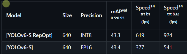
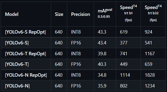
1 As of v0.2.0 release, traditional post-training quantization (PTQ) produces a degraded performance of YOLOv6-S from 43.4% to 41.2%.

​ 直接使用PTQ，精度降低了2.2%

2 We apply post-training quantization to YOLOv6-S-RepOpt, and its mAP slightly drops by 0.5%.

​ 使用了RepOPT、敏感性分析、PTQ之后，精度只降低了0.5%

3 Besides, we involve channel-wise distillation to accelerate the convergence. We finally reach a quantized model at 43.0% mAP. The performance arrives at 43.3% mAP, only 0.1% left to match the fully float precision of YOLOv6-S.

​ 再使用QAT中通道蒸馏加快收敛，精度提高了0.4%，最后只损失了0.1%的精度

Quantization-aware training (QAT)

1 Quantization Aware Training is based on Straight Through Estimator (STE) derivative approximation.

​ 量化感知训练是基于直通式估算器（STE）导数优化

2 After calibration is done, Quantization Aware Training is simply select a training schedule and continue training the calibrated model. Usually, it doesn’t need to fine tune very long. We usually use around 10% of the original training schedule, starting at 1% of the initial training learning rate, and a cosine annealing learning rate schedule that follows the decreasing half of a cosine period, down to 1% of the initial fine tuning learning rate (0.01% of the initial training learning rate).

​ 先标定int8，后QAT，二者需要互斥

​ 在训练的时候大概10%的epochs，学习率要小，初始学习率占1%，用cosine annealing learning衰减，知道学习率衰减到0.01%的初始学习率

3 Do not change quantization representation (scale) during training, at least not too frequently. Changing scale every step

​ 不要频繁的按照step改变学习率

• https://github.com/meituan/YOLOv6/blob/main/tools/qat/qat_utils.py

  • https://docs.nvidia.com/deeplearning/tensorrt/pytorch-quantization-toolkit/docs/userguide.html#quantization-aware-training

• 通道蒸馏 channel-wise kd

  • Channel-wise Knowledge Distillation for Dense Prediction

    • https://arxiv.org/abs/2011.13256

  • Spatial distillation：空间方向的蒸馏，可以理解成对所有通道的相同位置的点做归一化，然后让学生网络学习这个归一化后的分布，可以理解成对类别的蒸馏。

  • Channel distillation： 通道方向的蒸馏，可以理解成对单个通道内做归一化，然后让学生网络学习这个归一化后的分布，可以理解成对位置的蒸馏。

if self.args.distill:
    with torch.no_grad():
        t_preds, t_featmaps = self.teacher_model(images)
    temperature = self.args.temperature
    total_loss, loss_items = self.compute_loss_distill(preds, t_preds, s_featmaps, t_featmaps, targets, \
                                                      epoch_num, self.max_epoch, temperature, step_num,
                                                      batch_height, batch_width)

def distill_loss_cw(self, s_feats, t_feats,  temperature=1):
    N,C,H,W = s_feats[0].shape
    # print(N,C,H,W)
    loss_cw = F.kl_div(F.log_softmax(s_feats[0].view(N,C,H*W)/temperature, dim=2),
                       F.log_softmax(t_feats[0].view(N,C,H*W).detach()/temperature, dim=2),
                       reduction='sum',
                       log_target=True) * (temperature * temperature)/ (N*C)

    N,C,H,W = s_feats[1].shape
    # print(N,C,H,W)
    loss_cw += F.kl_div(F.log_softmax(s_feats[1].view(N,C,H*W)/temperature, dim=2),
                       F.log_softmax(t_feats[1].view(N,C,H*W).detach()/temperature, dim=2),
                       reduction='sum',
                       log_target=True) * (temperature * temperature)/ (N*C)

    N,C,H,W = s_feats[2].shape
    # print(N,C,H,W)
    loss_cw += F.kl_div(F.log_softmax(s_feats[2].view(N,C,H*W)/temperature, dim=2),
                       F.log_softmax(t_feats[2].view(N,C,H*W).detach()/temperature, dim=2),
                       reduction='sum',
                       log_target=True) * (temperature * temperature)/ (N*C)
    # print(loss_cw)
    return loss_cw

Export to ONNX

• 使用了pytorch_quantization后模型由pt导出onnx需要使用pytorch的伪量化函数

# First set static member of TensorQuantizer to use Pytorch’s own fake quantization functions
from pytorch_quantization import nn as quant_nn
quant_nn.TensorQuantizer.use_fb_fake_quant = True

Deployment with TensorRT

​ 最好用docker-TensorRT-8.5版本

• performance

• INT8 calibration

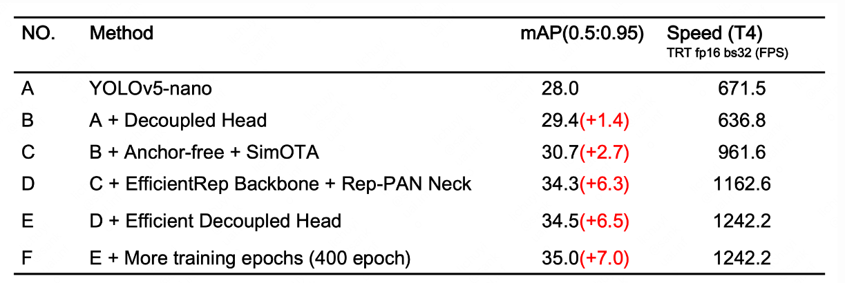
• ablation study for yolov6-nano

Notes

• 无论是PTQ推理量化，还是QAT训练量化，二者都需要对需要量化的层进行替换，最终保存是量化后网络的权重，而非网络结构
• 这篇文章工程能力很强，值得借鉴

References

• A Survey of Model Compression and Acceleration for Deep Neural Networks
• https://github.com/meituan/YOLOv6/blob/main/docs/tutorial_repopt.md