DDPM-Code

Denoising Diffusion Probabilistic Model | Code Analysis

---

• code https://github.com/lucidrains/denoising-diffusion-pytorch

---

Diffusion models

包括2个过程：

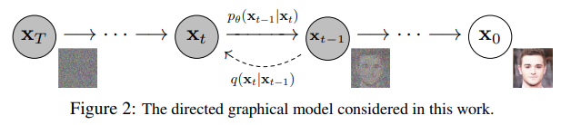
1. 前向加噪过程 q ：从数据分布中采样一张真实图像作为X0，通过有限个时间步T（T=1000），将从高斯分布采样的噪声不断叠加到真实图像中，直到第T次真实图像变成纯噪声图像XT。

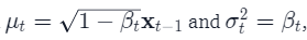
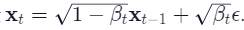
• e服从标准正态分布N(0,1)
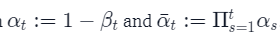
• 方差策略是0<β1<β2<…<βT<1，当β=0，Xt=X0，纯真实图像；当β=1，Xt=XT=e， 纯噪声

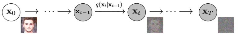
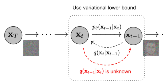
2. 反向去噪过程p_theta：训练一个神经网络用于学习所加噪声的分布，从而逐步将纯噪声图像XT反向去噪变成一个真实图像。

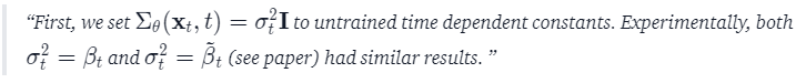
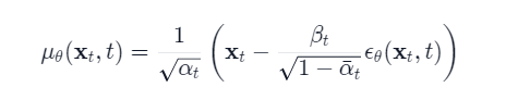
• 因为不知道条件分布 p(Xt-1 | Xt) ，所以需要神经网络拟合条件分布，只需要拟合分布的均值和标准差即可，采用梯度下降进行参数更新p_theta(Xt-1 | Xt)

• 原文只拟合了均值，方差固定，后来研究指出拟合方差会带来性能提升

Object function

• 扩散过程q和p_theta可以看做VAE，因此变分下界ELBO可以被用作最小化负对数似然函数，那么ELBO就是各个时间步损失函数之和。

• 通过重构扩散过程，除了L0以外，其它损失函数使用KL 散度度量2个高斯分布，即通过L2-loss优化均值

• 通过重参数化，实现直接从X0采样得到Xt，而不需要链式采样

• 神经网络（e_theta(Xt, t )）变成了所加噪声预测器，而不是均值预测器

• 最终，MSE损失函数如下

• e服从标准正态分布N（0,1）

Code analysis

Network helpers

首先，我们定义了一些辅助函数和类，这些函数和类将在实现神经网络时使用。重要的是，我们定义了一个 “残差”（Residual）模块，它可以简单地将输入添加到特定函数的输出中（换句话说，将残差连接添加到特定函数中）。我们还为上采样和下采样操作定义了别名。

def exists(x):
    return x is not None

def default(val, d):
    if exists(val):
        return val
    return d() if isfunction(d) else d


def num_to_groups(num, divisor):
    groups = num // divisor
    remainder = num % divisor
    arr = [divisor] * groups
    if remainder > 0:
        arr.append(remainder)
    return arr


class Residual(nn.Module):
    def __init__(self, fn):
        super().__init__()
        self.fn = fn

    def forward(self, x, *args, **kwargs):
        return self.fn(x, *args, **kwargs) + x


def Upsample(dim, dim_out=None):
    return nn.Sequential(
        nn.Upsample(scale_factor=2, mode="nearest"),
        nn.Conv2d(dim, default(dim_out, dim), 3, padding=1),
    )


def Downsample(dim, dim_out=None):
    # No More Strided Convolutions or Pooling
    return nn.Sequential(
        Rearrange("b c (h p1) (w p2) -> b (c p1 p2) h w", p1=2, p2=2),
        nn.Conv2d(dim * 4, default(dim_out, dim), 1),
    )

Position embeddings

由于神经网络的参数是跨时间（噪声水平）共享的，因此作者采用正弦位置嵌入来编码。这样，神经网络就能 “知道 “批次中的每张图像是在哪个特定的时间步长（噪声水平）下运行的。正弦位置嵌入（SinusoidalPositionEmbeddings）模块将形状张量（batch_size, 1）作为输入（即批次中若干噪声图像的噪声水平），并将其转化为形状张量（batch_size, dim），其中 dim 是位置嵌入的维度。然后将其添加到每个残差块中，我们将进一步了解这一点。

class SinusoidalPositionEmbeddings(nn.Module):
    def __init__(self, dim):
        super().__init__()
        self.dim = dim

    def forward(self, time):
        device = time.device
        half_dim = self.dim // 2
        embeddings = math.log(10000) / (half_dim - 1)
        embeddings = torch.exp(torch.arange(half_dim, device=device) * -embeddings)
        embeddings = time[:, None] * embeddings[None, :]
        embeddings = torch.cat((embeddings.sin(), embeddings.cos()), dim=-1)
        return embeddings

ResNet block

接下来，我们定义 U-Net 模型的核心构建模块。DDPM 的作者采用了一个宽 ResNet 模块，但 Phil Wang 用一个 “权重标准化 “版本取代了标准卷积层，该版本与组归一化相结合效果更好。

class WeightStandardizedConv2d(nn.Conv2d):
    """
    https://arxiv.org/abs/1903.10520
    weight standardization purportedly works synergistically with group normalization
    """

    def forward(self, x):
        eps = 1e-5 if x.dtype == torch.float32 else 1e-3

        weight = self.weight
        mean = reduce(weight, "o ... -> o 1 1 1", "mean")
        var = reduce(weight, "o ... -> o 1 1 1", partial(torch.var, unbiased=False))
        normalized_weight = (weight - mean) * (var + eps).rsqrt()

        return F.conv2d(
            x,
            normalized_weight,
            self.bias,
            self.stride,
            self.padding,
            self.dilation,
            self.groups,
        )


class Block(nn.Module):
    def __init__(self, dim, dim_out, groups=8):
        super().__init__()
        self.proj = WeightStandardizedConv2d(dim, dim_out, 3, padding=1)
        self.norm = nn.GroupNorm(groups, dim_out)
        self.act = nn.SiLU()

    def forward(self, x, scale_shift=None):
        x = self.proj(x)
        x = self.norm(x)

        if exists(scale_shift):
            scale, shift = scale_shift
            x = x * (scale + 1) + shift

        x = self.act(x)
        return x


class ResnetBlock(nn.Module):
    """https://arxiv.org/abs/1512.03385"""

    def __init__(self, dim, dim_out, *, time_emb_dim=None, groups=8):
        super().__init__()
        self.mlp = (
            nn.Sequential(nn.SiLU(), nn.Linear(time_emb_dim, dim_out * 2))
            if exists(time_emb_dim)
            else None
        )

        self.block1 = Block(dim, dim_out, groups=groups)
        self.block2 = Block(dim_out, dim_out, groups=groups)
        self.res_conv = nn.Conv2d(dim, dim_out, 1) if dim != dim_out else nn.Identity()

    def forward(self, x, time_emb=None):
        scale_shift = None
        if exists(self.mlp) and exists(time_emb):
            time_emb = self.mlp(time_emb)
            time_emb = rearrange(time_emb, "b c -> b c 1 1")
            scale_shift = time_emb.chunk(2, dim=1)

        h = self.block1(x, scale_shift=scale_shift)
        h = self.block2(h)
        return h + self.res_conv(x)

Attention module

接下来，我们定义 DDPM 作者在卷积模块之间添加的注意力模块。Phil Wang 采用了两种注意力变体：一种是常规的多头自我注意力（如 Transformer 中使用的那样），另一种是线性注意力变体，其时间和内存要求与序列长度成线性比例，而常规注意力则为二次。

class Attention(nn.Module):
    def __init__(self, dim, heads=4, dim_head=32):
        super().__init__()
        self.scale = dim_head**-0.5
        self.heads = heads
        hidden_dim = dim_head * heads
        self.to_qkv = nn.Conv2d(dim, hidden_dim * 3, 1, bias=False)
        self.to_out = nn.Conv2d(hidden_dim, dim, 1)

    def forward(self, x):
        b, c, h, w = x.shape
        qkv = self.to_qkv(x).chunk(3, dim=1)
        q, k, v = map(
            lambda t: rearrange(t, "b (h c) x y -> b h c (x y)", h=self.heads), qkv
        )
        q = q * self.scale

        sim = einsum("b h d i, b h d j -> b h i j", q, k)
        sim = sim - sim.amax(dim=-1, keepdim=True).detach()
        attn = sim.softmax(dim=-1)

        out = einsum("b h i j, b h d j -> b h i d", attn, v)
        out = rearrange(out, "b h (x y) d -> b (h d) x y", x=h, y=w)
        return self.to_out(out)

class LinearAttention(nn.Module):
    def __init__(self, dim, heads=4, dim_head=32):
        super().__init__()
        self.scale = dim_head**-0.5
        self.heads = heads
        hidden_dim = dim_head * heads
        self.to_qkv = nn.Conv2d(dim, hidden_dim * 3, 1, bias=False)

        self.to_out = nn.Sequential(nn.Conv2d(hidden_dim, dim, 1), 
                                    nn.GroupNorm(1, dim))

    def forward(self, x):
        b, c, h, w = x.shape
        qkv = self.to_qkv(x).chunk(3, dim=1)
        q, k, v = map(
            lambda t: rearrange(t, "b (h c) x y -> b h c (x y)", h=self.heads), qkv
        )

        q = q.softmax(dim=-2)
        k = k.softmax(dim=-1)

        q = q * self.scale
        context = torch.einsum("b h d n, b h e n -> b h d e", k, v)

        out = torch.einsum("b h d e, b h d n -> b h e n", context, q)
        out = rearrange(out, "b h c (x y) -> b (h c) x y", h=self.heads, x=h, y=w)
        return self.to_out(out)

Group normalization

DDPM 作者将 U-Net 的卷积层/注意力层与组规范化交错在一起（。下面，我们定义了一个 PreNorm 类，它将用于在注意力层之前应用组归一化，我们将进一步了解。请注意，关于在 Transformers 中是在注意力之前还是之后应用归一化，一直存在争议。

class PreNorm(nn.Module):
    def __init__(self, dim, fn):
        super().__init__()
        self.fn = fn
        self.norm = nn.GroupNorm(1, dim)

    def forward(self, x):
        x = self.norm(x)
        return self.fn(x)

Conditional U-Net

现在，我们已经定义了所有构建模块（位置嵌入、ResNet 模块、注意力和组归一化），是时候定义整个神经网络了。 神经网络接收一批噪声图像及其各自的噪声水平，并输出添加到输入图像中的噪声。

• 网络将一批形状为（batch_size、num_channels、height、width）的噪声图像和一批形状为（batch_size、1）的噪声级别作为输入，并返回一个形状为（batch_size、num_channels、height、width）的张量。

U-Net网络构建过程如下：

• 首先，在一批噪声图像上应用卷积层，并根据噪声水平计算位置嵌入值
• 然后，应用一系列降采样阶段。每个降采样阶段包括 2 ResNet blocks + groupnorm + attention + residual connection + a downsample
• 在网络中间，再次应用 ResNet 块，并与注意力交错进行
• 接下来是一连串的上采样阶段。每个上采样阶段由 2 ResNet blocks + groupnorm + attention + residual connection + an upsample operation
• 最后，应用一个 ResNet 块和一个卷积层。

class Unet(nn.Module):
    def __init__(
        self,
        dim,
        init_dim=None,
        out_dim=None,
        dim_mults=(1, 2, 4, 8),
        channels=3,
        self_condition=False,
        resnet_block_groups=4,
    ):
        super().__init__()

        # determine dimensions
        self.channels = channels
        self.self_condition = self_condition
        input_channels = channels * (2 if self_condition else 1)

        init_dim = default(init_dim, dim)
        self.init_conv = nn.Conv2d(input_channels, init_dim, 1, padding=0) # changed to 1 and 0 from 7,3

        dims = [init_dim, *map(lambda m: dim * m, dim_mults)]
        in_out = list(zip(dims[:-1], dims[1:]))

        block_klass = partial(ResnetBlock, groups=resnet_block_groups)

        # time embeddings
        time_dim = dim * 4

        self.time_mlp = nn.Sequential(
            SinusoidalPositionEmbeddings(dim),
            nn.Linear(dim, time_dim),
            nn.GELU(),
            nn.Linear(time_dim, time_dim),
        )

        # layers
        self.downs = nn.ModuleList([])
        self.ups = nn.ModuleList([])
        num_resolutions = len(in_out)

        for ind, (dim_in, dim_out) in enumerate(in_out):
            is_last = ind >= (num_resolutions - 1)

            self.downs.append(
                nn.ModuleList(
                    [
                        block_klass(dim_in, dim_in, time_emb_dim=time_dim),
                        block_klass(dim_in, dim_in, time_emb_dim=time_dim),
                        Residual(PreNorm(dim_in, LinearAttention(dim_in))),
                        Downsample(dim_in, dim_out)
                        if not is_last
                        else nn.Conv2d(dim_in, dim_out, 3, padding=1),
                    ]
                )
            )

        mid_dim = dims[-1]
        self.mid_block1 = block_klass(mid_dim, mid_dim, time_emb_dim=time_dim)
        self.mid_attn = Residual(PreNorm(mid_dim, Attention(mid_dim)))
        self.mid_block2 = block_klass(mid_dim, mid_dim, time_emb_dim=time_dim)

        for ind, (dim_in, dim_out) in enumerate(reversed(in_out)):
            is_last = ind == (len(in_out) - 1)

            self.ups.append(
                nn.ModuleList(
                    [
                        block_klass(dim_out + dim_in, dim_out, time_emb_dim=time_dim),
                        block_klass(dim_out + dim_in, dim_out, time_emb_dim=time_dim),
                        Residual(PreNorm(dim_out, LinearAttention(dim_out))),
                        Upsample(dim_out, dim_in)
                        if not is_last
                        else nn.Conv2d(dim_out, dim_in, 3, padding=1),
                    ]
                )
            )

        self.out_dim = default(out_dim, channels)

        self.final_res_block = block_klass(dim * 2, dim, time_emb_dim=time_dim)
        self.final_conv = nn.Conv2d(dim, self.out_dim, 1)

    def forward(self, x, time, x_self_cond=None):
        if self.self_condition:
            x_self_cond = default(x_self_cond, lambda: torch.zeros_like(x))
            x = torch.cat((x_self_cond, x), dim=1)

        x = self.init_conv(x)
        r = x.clone()

        t = self.time_mlp(time)

        h = []

        for block1, block2, attn, downsample in self.downs:
            x = block1(x, t)
            h.append(x)

            x = block2(x, t)
            x = attn(x)
            h.append(x)

            x = downsample(x)

        x = self.mid_block1(x, t)
        x = self.mid_attn(x)
        x = self.mid_block2(x, t)

        for block1, block2, attn, upsample in self.ups:
            x = torch.cat((x, h.pop()), dim=1)
            x = block1(x, t)

            x = torch.cat((x, h.pop()), dim=1)
            x = block2(x, t)
            x = attn(x)

            x = upsample(x)

        x = torch.cat((x, r), dim=1)

        x = self.final_res_block(x, t)
        return self.final_conv(x)

Defining the forward diffusion process

def cosine_beta_schedule(timesteps, s=0.008):
    """
    cosine schedule as proposed in https://arxiv.org/abs/2102.09672
    """
    steps = timesteps + 1
    x = torch.linspace(0, timesteps, steps)
    alphas_cumprod = torch.cos(((x / timesteps) + s) / (1 + s) * torch.pi * 0.5) ** 2
    alphas_cumprod = alphas_cumprod / alphas_cumprod[0]
    betas = 1 - (alphas_cumprod[1:] / alphas_cumprod[:-1])
    return torch.clip(betas, 0.0001, 0.9999)

def linear_beta_schedule(timesteps):
    beta_start = 0.0001
    beta_end = 0.02
    return torch.linspace(beta_start, beta_end, timesteps)

def quadratic_beta_schedule(timesteps):
    beta_start = 0.0001
    beta_end = 0.02
    return torch.linspace(beta_start**0.5, beta_end**0.5, timesteps) ** 2

def sigmoid_beta_schedule(timesteps):
    beta_start = 0.0001
    beta_end = 0.02
    betas = torch.linspace(-6, 6, timesteps)
    return torch.sigmoid(betas) * (beta_end - beta_start) + beta_start



timesteps = 300

# define beta schedule
betas = linear_beta_schedule(timesteps=timesteps)

# define alphas 
alphas = 1. - betas
alphas_cumprod = torch.cumprod(alphas, axis=0)
alphas_cumprod_prev = F.pad(alphas_cumprod[:-1], (1, 0), value=1.0)
sqrt_recip_alphas = torch.sqrt(1.0 / alphas)

# calculations for diffusion q(x_t | x_{t-1}) and others
sqrt_alphas_cumprod = torch.sqrt(alphas_cumprod)
sqrt_one_minus_alphas_cumprod = torch.sqrt(1. - alphas_cumprod)

# calculations for posterior q(x_{t-1} | x_t, x_0)
posterior_variance = betas * (1. - alphas_cumprod_prev) / (1. - alphas_cumprod)

def extract(a, t, x_shape):
    batch_size = t.shape[0]
    out = a.gather(-1, t.cpu())
    return out.reshape(batch_size, *((1,) * (len(x_shape) - 1))).to(t.device)

Training algorithm

算法过程：

• 从标准高斯分布采样一个噪声e
• 通过梯度下降最小化损失
• 训练到收敛为止（训练时间比较长，T 代码中设置为 1000）

Denoising sampling

可以利用神经网络噪声预测器，通过插入平均值的重参数化，得到一个去噪程度稍低的图像 Xt-1

算法过程：

• 从标准高斯分布采样一个噪声
• 从时间步 T 开始正向扩散迭代到时间步 1
• 如果时间步不为 1，则从标准高斯分布采样一个噪声 z
• 根据高斯分布计算每个时间步 t 的噪声图

@torch.no_grad()
def p_sample(model, x, t, t_index):
    betas_t = extract(betas, t, x.shape)
    sqrt_one_minus_alphas_cumprod_t = extract(
        sqrt_one_minus_alphas_cumprod, t, x.shape
    )
    sqrt_recip_alphas_t = extract(sqrt_recip_alphas, t, x.shape)
    
    # Equation 11 in the paper
    # Use our model (noise predictor) to predict the mean
    model_mean = sqrt_recip_alphas_t * (
        x - betas_t * model(x, t) / sqrt_one_minus_alphas_cumprod_t
    )

    if t_index == 0:
        return model_mean
    else:
        posterior_variance_t = extract(posterior_variance, t, x.shape)
        noise = torch.randn_like(x)
        # Algorithm 2 line 4:
        return model_mean + torch.sqrt(posterior_variance_t) * noise 

# Algorithm 2 (including returning all images)
@torch.no_grad()
def p_sample_loop(model, shape):
    device = next(model.parameters()).device

    b = shape[0]
    # start from pure noise (for each example in the batch)
    img = torch.randn(shape, device=device)
    imgs = []

    for i in tqdm(reversed(range(0, timesteps)), desc='sampling loop time step', total=timesteps):
        img = p_sample(model, img, torch.full((b,), i, device=device, dtype=torch.long), i)
        imgs.append(img.cpu().numpy())
    return imgs

@torch.no_grad()
def sample(model, image_size, batch_size=16, channels=3):
    return p_sample_loop(model, shape=(batch_size, channels, image_size, image_size))

Experimental results

Note

• @property装饰器把方法变成属性，不可调用（不加（）），作用是防止方法被修改——变成只读
• FID(Frechet Inception Distance score)图像生成质量评价指标，较低的FID意味着生成分布与真实图片分布之间更接近

Conclusions

1. Diffusion Model 通过参数化的方式表示为马尔科夫链，这意味着隐变量Xt都满足当前时间步t只依赖于上一个时间步t-1
2. 马尔科夫链中的转变概率分布 p_theta 服从高斯分布，在正向扩散过程当中高斯分布的参数是直接设定的，而逆向过程中的高斯分布参数是通过学习得到的
3. Diffusion Model 网络模型扩展性和鲁棒性比较强，可以选择输入和输出维度相同的网络模型，例如类似于UNet的架构，保持网络模型的输入和输出 Tensor dims 相等
4. Diffusion Model 的目的是对输入数据求极大似然函数，实际表现为通过训练来调整模型参数以最小化数据的负对数似然的变分上限
5. 在概率分布转换过程中，因为通过马尔科夫假设，目标函数中的变分上限都可以转变为利用 KL 散度来计算，因此避免了采用蒙特卡洛采样的方式